Posted by: christian on 22 Jan 2021
Just a quick demonstration of using Matplotlib and Pillow to customize a chart in the style of a 1950s academic journal article.
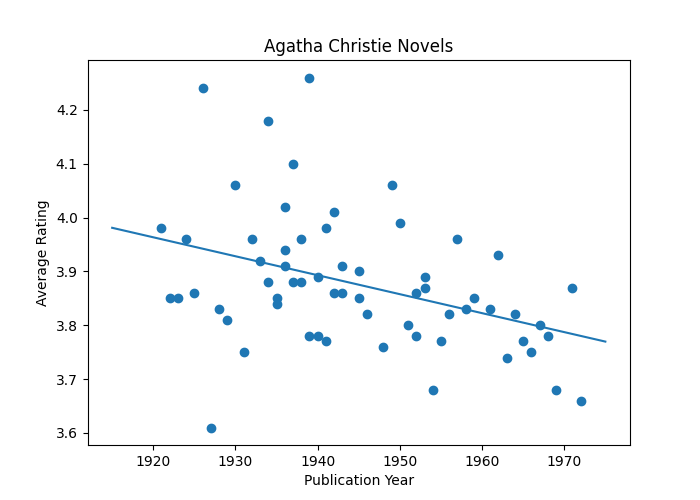
The default Matplotlib styles are pleasing enough (here the scatter plot is of data taken from the file ac-ratings-gr.csv).
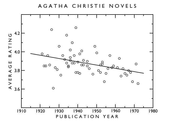
Some 1950s academic journal style (think: lettering guides and French curves) can be introduced with some judiciously-chosen Matplotlib styles. First, old-style.mplstyle:
axes.linewidth : 1.5
xtick.labelsize : 11
ytick.labelsize : 11

lines.linewidth : 1.5
lines.markersize : 6
lines.markerfacecolor: white
lines.markeredgecolor: k

xtick.major.size: 10
xtick.major.width: 1.5
xtick.minor.size: 4
xtick.minor.width: 1.5
xtick.direction: in
xtick.major.pad: 5

ytick.major.size: 10
ytick.major.width: 1.5
ytick.minor.size: 4
ytick.minor.width: 1.5
ytick.direction: in

axes.titleweight: normal
axes.titlepad: 20
Next, some customization and the timeless (unlike its creator) font, Gill Sans. Matplotlib has a hard time dealing with system fonts on some platforms (such as mine, macOS), so point the FontProperties fname argument wherever the font lives in your filesystem.
import numpy as np
import pandas as pd
from sklearn.linear_model import LinearRegression
import matplotlib.font_manager as fm
import matplotlib.pyplot as plt
from matplotlib.ticker import MultipleLocator

gs_font = fm.FontProperties(
                fname='/System/Library/Fonts/Supplemental/GillSans.ttc')

plt.style.use('./old-style.mplstyle')

df = pd.read_csv('ac-ratings-gr.csv', header=1, index_col=0)

# Drop the mid-career novels published in the '70s and low-quality outliers.
df = df.drop(['Curtain', 'Sleeping Murder',
               'Passenger to Frankfurt', 'Postern of Fate'])
# We require column vectors (n, 1) for the data, so add an axis.
X = df.loc[:, "Publication Year"].values[:, None]
Y = df.loc[:, "Average Rating"].values[:, None]

linear_regressor = LinearRegression()
reg = linear_regressor.fit(X, Y)

WIDTH, HEIGHT, DPI = 700, 500, 100
fig, ax = plt.subplots(figsize=(WIDTH/DPI, HEIGHT/DPI), dpi=DPI)

ax.scatter(X, Y, color=[0,0,0,0], edgecolors='k')
Xpred = np.linspace(1915, 1975, 2)[:, None]
Ypred = linear_regressor.predict(Xpred)
ax.plot(Xpred, Ypred, 'k')
ax.xaxis.set_minor_locator(MultipleLocator(5))
ax.yaxis.set_minor_locator(MultipleLocator(0.1))
ax.set_xlabel(' '.join('PUBLICATION YEAR'), fontproperties=gs_font,
              fontsize=14)
ax.set_ylabel(' '.join('AVERAGE RATING'), fontproperties=gs_font, fontsize=14)
ax.set_xlim(1910, 1980)
ax.set_ylim(3.4, 4.4)
ax.set_yticks([3.6, 3.8, 4.0, 4.2])
ax.tick_params('x', which='both', top=True, bottom=True)
ax.tick_params('y', which='both', right=True, left=True)

for tick in ax.get_xticklabels():
    tick.set_fontname("Gill Sans")
    tick.set_fontsize(14)
for tick in ax.get_yticklabels():
    tick.set_fontname("Gill Sans")
    tick.set_fontsize(14)


ax.set_title(' '.join('AGATHA CHRISTIE NOVELS'), fontproperties=gs_font,
             fontsize=16)

plt.savefig('ag-ratings.png', dpi=DPI)
plt.show()
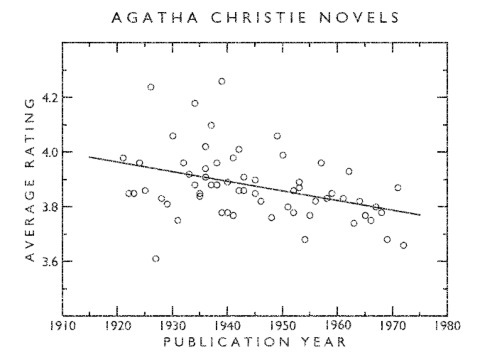
Finally, to add an authentic "photocopied a few too many times" look, add some noise and blur with this small module, add_noise.py:
from functools import partial
from random import gauss, randrange
from PIL import Image, ImageFilter

def add_noise_to_image(im, perc=20, blur=0.5):
    gaussian = partial(gauss, 0.50, 0.02)
    width, height = im.size
    for _ in range(width*height * perc // 100):
        noise = int(gaussian() * 255)
        x, y = randrange(width), randrange(height)
        r, g, b, a = im.getpixel((x, y))
        im.putpixel((x, y),
                    (min(r+noise, 255), min(g+noise, 255), min(b+noise, 255)))

    im = im.filter(ImageFilter.GaussianBlur(blur))
    return im
It is used as follows on the plot image just created:
from PIL import Image
from add_noise import add_noise_to_image

im = Image.open('ag-ratings.png')
im = add_noise_to_image(im, 40)
im.save('ag-ratings-noisy.png')
im.show()
Comments
Comments are pre-moderated. Please be patient and your comment will appear soon.
There are currently no comments
New Comment